The topic that we are going to deal with next has to do with exoplanets, specifically with the observation of transits of exoplanets, but I will include a proposal, or describe a technique, that can be used by non-professional astronomers, and whose results could go in line with the characterization of planetary atmospheres.
I understand that the reader knows what an exoplanet is, what a transit is and how to observe it, even so we will see an introduction to it and attach a link that refers to a tutorial in which we explain how to make this type of observations. Exoplanets.pdf
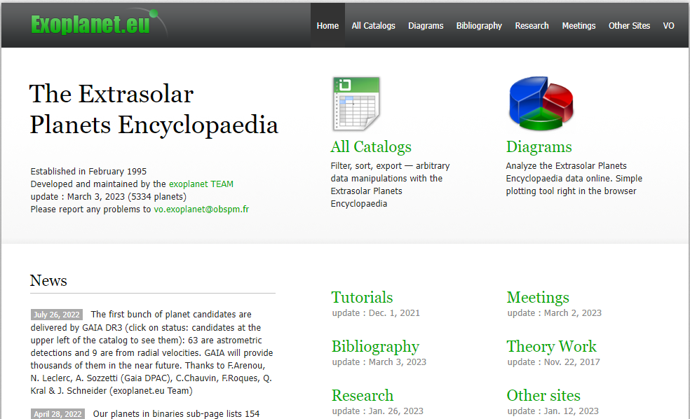
We call exoplanets to planets that are revolving around other stars other than the sun, they are planets in other solar systems around other stars, the first exoplanet discovered, although there is a long history of detections, was discovered in 1994 and was presented in 1995, that is, relatively recently and since then to date more than 5,000 planets are known in other stars, As can be seen in the following image taken from the database of http://exoplanet.eu/.
These planets have been discovered since 1995 applying different techniques, however, the technique that has been most successful and the one that has allowed to find most of the exoplanets that we know today, is the photometric technique or technique of exoplanetary transits.
Thanks to all the experiments and missions, today we know about 5,000 exoplanets and more than 600 multiple planetary systems.
The first exoplanets by the transit technique, were discovered from ground-based observatories however, it has been the advent of space observatories such as Kepler or TESS for the detection of extra-solar planets with this method of transits, which allowed to greatly increase the number of known exoplanets, in fact, well over half of confirmed exoplanets have been found through observations by the transit technique.
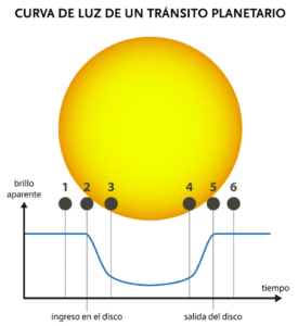
An exoplanet transit occurs when the planet comes between the observer and the central star of the system, the planet obscures a small fraction of its star’s brightness, assuming that in the short term the star does not vary much. In a brief summary, we see that before the transit occurs the brightness of the star is constant, when the planet begins to come between the star and the observer the brightness of the star decreases, and when the planet has been completely introduced in front of the disk of its star then we see that the decrease in brightness is important.
The observation of exoplanet transits has become an activity or a discipline that amateur or non-professional astronomers practice successfully and with solvency, usually focused on Jupiter-type giant planets.
Transits usually occur whose depth and amplitude of the observed variation is thousandths of magnitude, this is a very small amplitude, but who already has training in the observation of variable stars with variations of one to two hundredths of magnitude for example, can enter this technique of differential photometry.
The means available to amateurs and also the training of them in relatively complex techniques of both observation and data reduction, allow to achieve lower precisions, well below the hundredth of magnitude.
The growing number of amateur astronomers who observe and record these transits of exoplanets has led to organizations or institutions that centralize and collect all these data obtained from observations of transits, as an example and perhaps the reference in this type of observations. Exoplanet Transit Database or ETD of the Astronomical Society of the Czech Republic, which collects all the transits that observers send to this organization. Another example of collaboration and use of data by professional projects is ExoClock, dedicated to the calculation of TTV’s (Transit Time Variations) in collaboration with ESA’s future ARIEL probe that will study, what exoplanets are made of, how they formed and how they evolved, examining a diverse sample of around 1000 extrasolar planets.
Normally what we do is observe exoplanets that are already known and the regular observation of transits of known exoplanets has scientific utility such as the control of the orbital period of the planets. That is, knowing the period of the exoplanet and knowing the time in which it has occurred we can infer, since it is a periodic phenomenon and we know when the next transit will take place, we see that the difference in the transit time we observe and the time predicted by that ephemeris is close to zero, then we conclude that the ephemeris is correct and that the orbital period is stable and therefore we have controlled the planet as a planet in a regular orbit. In some cases anomalies can be detected in this relationship and it can be detected that sometimes the observed transit is advanced or delayed with respect to the expected time and that indicates anomalies in the orbit of that planet, this technique is called TTV’s (Transit Time Variations).
These anomalies may be due, on the one hand, to the presence of other planets in the system, which by gravitational attraction disturb the orbit of the known exoplanet and in fact the observation of these variations in transit times have served to propose and even detect the presence of new planets in already known planetary systems, and that they had not been previously detected by either photometric technique, spectroscopic technique, or any other technique.
A periodic variation in the advance or delay of maximum time could also indicate the presence of a satellite on this planet although we do not know that any exomoon has been discovered with this technique.
However, despite the interest of all this, what we are going to expose here is another type of observation that could provide us with new data about the planet we are observing and in particular data related to its atmosphere and this could be obtained as it has already been obtained in some cases by studying the transits of the exoplanet in a photometric way, but using different photometric filters.
Here we have, for example, observations of the transit of an exoplanet, wasp-12b obtained with different photometric filters.
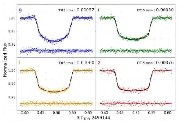
The points are obtained from different photometric filters sloan g, r, i and z, we see that apparently in this curve, the depth of the transit observed in the g filter seems to be greater than the depth of the transit observed in the r filter.
How can it be? Why, of course, if we consider that the disk is completely homogeneous and that the planet is completely opaque, let’s say that the effect of the transit would be purely geometric. The depth of the transit will be determined by the relationship between the size of the planet and the size of the star. However, this is not always the case, here are two examples. arxiv.org/abs/1603.02587 , arxiv.org/abs/1511.05601 Both are professional works, where the observations of transits are presented by means of the photometric technique and where it is observed that using different photometric filters the depth of the transit varies from one filter to another and how these authors interpret it, in particular how they interpret that difference in depth between the transits, when we observe with different filters.
Researchers interpret it, due to the presence of rayleigh scattering in the exoplanet’s atmosphere. Let’s explain this in a little more detail.
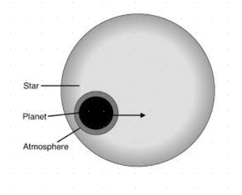
In this example, let’s say approximate, the transit is not only of the planet but of the planet with its atmosphere and if that atmosphere is transparent, like the atmosphere of the earth, then in that atmosphere like the atmosphere of the earth the rayleigh scattering will occur.
Rayleigh scattering is evident to the naked eye in the earth’s atmosphere and has several effects. It is produced by the fact that the light that reaches us from the sun, the photons that reach us from the sun interact with electrons of the atoms that are present in the atmosphere and then collide with the electrons of the atmosphere. These photons are scattered in a different direction than the one they impinge. This causes a phenomenon known as atmospheric extinction phenomenon, this rayleigh scattering is proportional to the wavelength of radiation raised to power minus 4, that is, it has a very large dependence on color and the shorter the wavelength of radiation, the bluer the light, The more it is subjected to Rayleigh scattering, and the redder the light, the less it is affected by scattering.
What would happen on a planet where we had a transparent atmosphere similar to Earth’s?
Well, we would have that the disk of the planet or the opaque areas of it would hide the light of the star in the same way, however, the atmosphere of the star also hides part of the radiation that comes from the star, but not in all wavelengths equally. So at the bluest wavelengths, there would be much more light scattered by the planet’s atmosphere, and therefore less would reach us at the redder wavelengths. The planet would apparently be larger when we observe it with a blue filter than when we observe it with a red filter.
In this way, if we see that in the bluest filters, the transit is deeper than in the redder filters, then we conclude that this is a transparent atmosphere in which the rayleigh scattering takes place.
What would be the alternative to an opaque atmosphere, for example an atmosphere completely covered with clouds?
In an atmosphere completely covered with clouds the atmosphere would be just as opaque as the disk of the planet, so an opaque atmosphere would do, as if the planet were larger, but in all filters, In this case, we would not find any difference in the depth of the transit between the bluest filters and the redder filters.
We propose that amateurs who may have interest, carry out tests of this type. Observe transits at various wavelengths and study whether this effect is seen, in which it is observed that transits taken with bluer filters are deeper than transits taken with redder filters. If we can conclude this, through the observation of several transits we can conclude that indeed that planet has a transparent atmosphere in which the scattering of rayleigh occurs.
However, if someone decides to tackle this research program, they should know that it is a rather complex program, because it is not enough to measure the depth of the transit really in different filters only. Since how it appears in this study arxiv.org/abs/1511.05601 The conclusion reached by the researchers is that the data which allows them to affirm that the atmosphere is transparent and subjected to Rayleigh scattering, is obtained when we measure the size of the planet through blue filters, a value significantly higher than when we measure the size of the planet through the reddest filters. And it is therefore necessary to determine the relative size of the planet with respect to the star.
It is not enough to directly compare the light curves and see if one is deeper than the other, because if we do so there may be another effect. and that it has nothing to do with the atmosphere of the planet that can influence us. This is the effect that is known as edge darkening or limb-darkening. In the following link you will find more information about this effect and how it affects the observations of transits. limb-darkening-exoplanets.
What is edge darkening orlimb-darkening?
If we look at this photograph of the sun taken during the transit of Venus we see that the part of the star closest to the limb looks redder, that is, less light arrives than from the central part and this is due to something similar to what we saw previously.
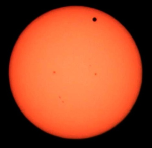
The scattering of the earth’s atmosphere causes the central parts of the sun or the light that comes out of the photosphere of a star, when we look in the central regions, we see that the thickness of the atmosphere crossed has been less, therefore, we see the brightest star per unit of surface, than when we approach the limb and see it reddish and less bright, Why? Because again the light that leaves this part of the photosphere of the sun, comes towards us in a way, so to speak, grazing with respect to the photosphere and crosses much more atmosphere, therefore, arrives more reddened.
If we now approach our project of trying to compare light curves taken in different filters, it turns out that this darkening at the edge or limb-darkening depends on the wavelength of the radiation, and is more noticeable for blue filters and less noticeable for redder filters. Because, it’s something like the scattering of the star’s own atmosphere, then.
What happens if we only compare depths of the transits we observe?
Well, we can observe variations that may be due to the difference in color of the darkening at the edge, and not really because the exoplanet has an atmosphere in which rayleigh scattering occurs.
So if we want to address this problem, if we want to try to detect transparent atmospheres and differentiate them from opaque atmospheres. What we would have to do is, from our observations, try to determine the relative size of the planet to its star, or the absolute size if we know the estimated size. And we can do this because, although it is a very complicated calculation from our light curve, calculate the intrinsic size of the planet, or the size of the exoplanet relative to the size of the star. However, there are tools on the network that can serve us for this purpose and can allow us to calculate several parameters of the exoplanet from our observed transit data.
From our light curve of a transit climbed for example to ETD, as we see in the previous graphs, we draw an average curve adjusted to the transit correcting the extinction and that average curve is parameterized by the physical parameters of the planet and its star.
One of those parameters that parameterizes the curve is the size of the planet, however, there is a much more efficient and easier to use tool that I recommend. It is the exo-fast tool that is available in NASA’s exoplanet archive: exoplanetarchive.ipac.caltech.edu/cgi-bin/ExoFAST/nph-exofast
We introduce some parameters related to the star but many of those parameters are known parameters that are incorporated into the tool itself, and others if they are not incorporated, can be searched in the exoplanet database. Later we will see how to use this tool.
Conclusions
So and by way of conclusion, to address a research project of this type what we would have to do is, first of all from the observational point of view, try to observe transits of exoplanets using several photometric filters, depending on the size of our telescope and how fast we can take the images. Short exposure times of the same transit will allow alternating between two photometric filters or you can also observe several transits of the same planet sometimes with one filter and sometimes with another.
In any case, even if we use these types of tools, the results are affected by a relatively large error because the depth of transit is small. Let’s say that to undertake a program of this type, we would have to consider systematically observing the same transits of exoplanets, to see if in any of them we actually detect this effect.
And to detect this effect the strategy would be, once the light curve is obtained, to make use of the exo-fast tool and from our light curve that we introduce into the tool, it will present us with the data and in particular we are interested in the data related to the size of the exoplanet.
But we will see all this in the next post, I hope it has been helpful.